Week 11

Blog sheet Week 11: Strain Gauges

Part A: Strain Gauges:

Strain gauges are used to measure the strain or stress levels on the materials. Alternatively, pressure on the strain gauge causes a generated voltage and it can be used as an energy harvester. You will be given either the flapping or tapping type gauge. When you test the circle buzzer type gauge, you will lay it flat on the table and tap on it. If it is the long rectangle one, you will flap the piece to generate voltage.

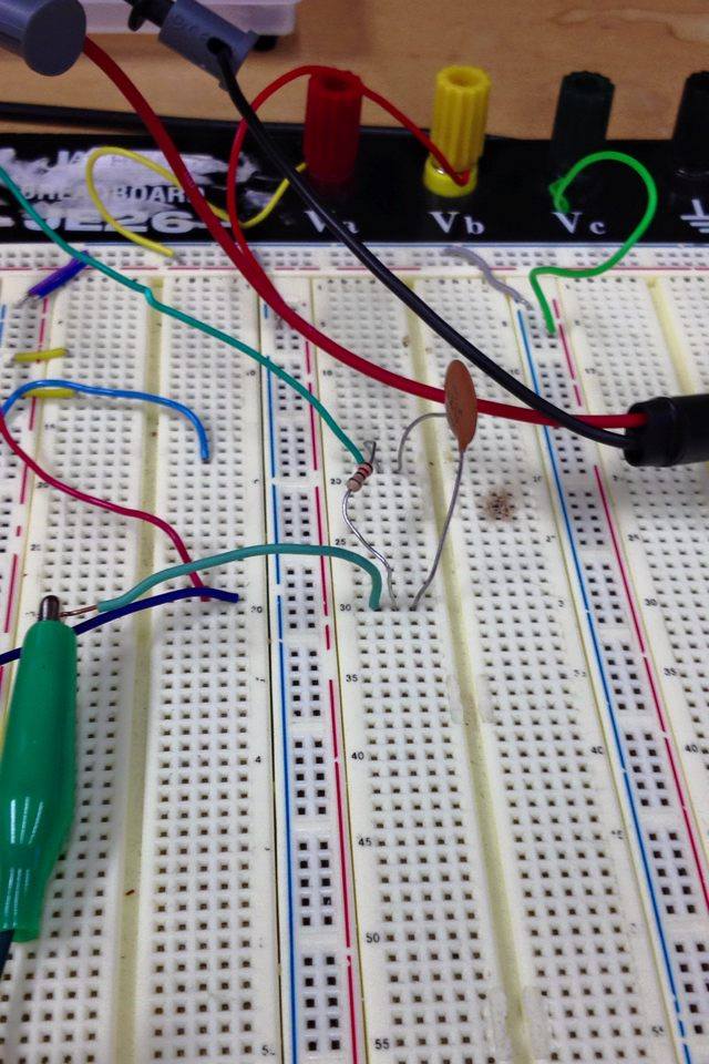
1.       Connect the oscilloscope probes to the strain gauge. Record the peak voltage values (positive and negative) by flipping/tapping the gauge with low and high pressure. Make sure to set the oscilloscope horizontal and vertical scales appropriately so you can read the values. DO NOT USE the measure tool of the oscilloscope. Adjust your oscilloscope so you can read the values from the screen. Fill out Table 1 and provide photos of the oscilloscope.

Table 1: Strain gauge characteristics

Flipping strength	Minimum Voltage	Maximum Voltage
Low	-380mV	4V
High	1V	35V

2.       Press the “Single” button below the Autoscale button on the oscilloscope. This mode will allow you to capture a single change at the output. Adjust your time and amplitude scales so you have the best resolution for your signal when you flip/tap your strain gauge. Provide a photo of the oscilloscope graph.

Part B: Half-Wave Rectifiers

1.       Construct the following half-wave rectifier. Measure the input and the output using the oscilloscope and provide a snapshot of the outputs.

2.       Calculate the effective voltage of the input and output and compare the values with the measured ones by completing the following table.

Effective (rms) values	Calculated	Measured
Input	3.536V	3.535V
Output	1.5916V	1.696V

3.       Construct the following circuit and record the output voltage using both DMM and the oscilloscope.

	Oscilloscope	DMM
Output Voltage (p-p)	.848V	Not Possible
Output Voltage (mean)	1.72V	Not Possible

4.       Replace the 1 µF capacitor with 100 µF and repeat the previous step. What has changed?

Since no 100 µF capacitor was available, we were provided with a 470 µF capacitor.  This is a much larger capacitor and means that we would not see the cap discharge at 1KHz.  In order to fix this we had to turn the frequency down.  In this case we used 6.3 Hz. 

	Oscilloscope	DMM
Output Voltage (p-p)	920mv	Not Possible
Output Voltage (mean)	5.67V	Not Possible

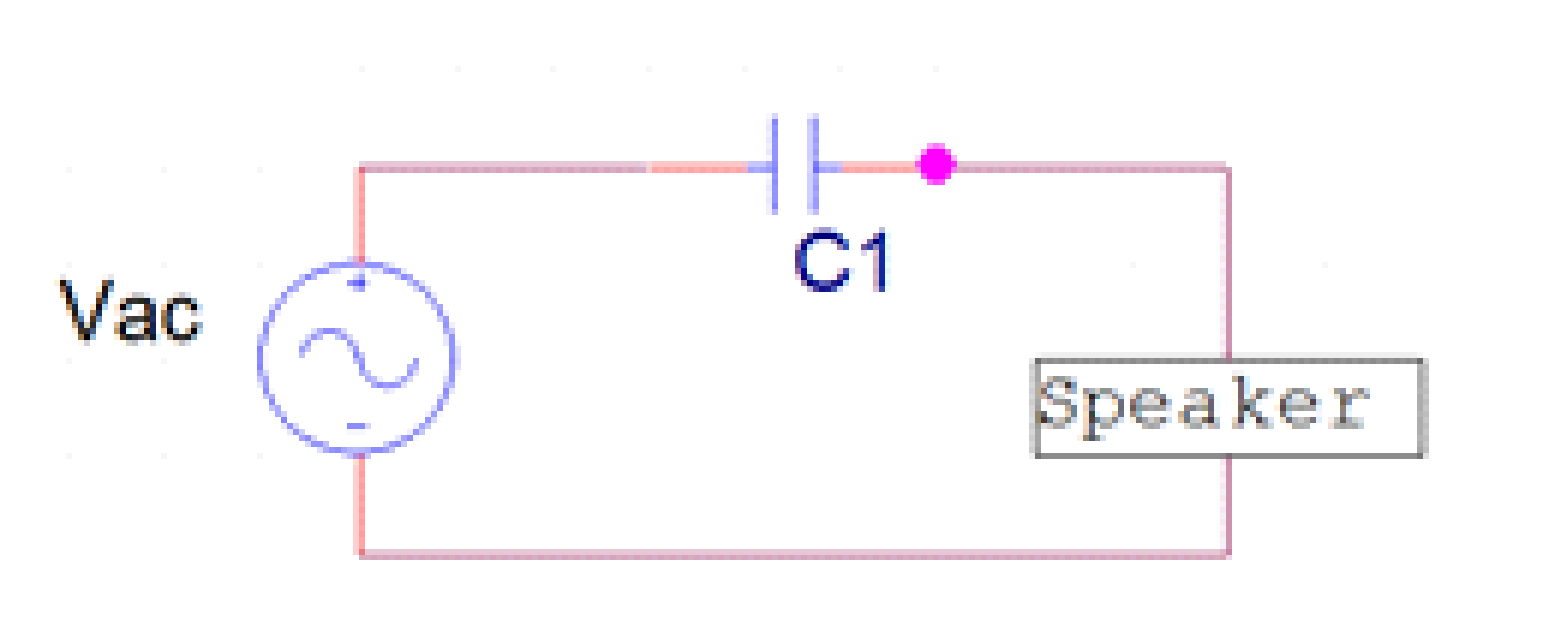
Part C: Energy Harvesters

1.       Construct the half-wave rectifier circuit without the resistor but with the 1 µF capacitor. Instead of the function generator, use the strain gauge. Discharge the capacitor every time you start a new measurement. Flip/tap your strain gauge and observe the output voltage. Fill out the table below:

Tap frequency	Duration	Output voltage
1 flip/second	10 seconds	5.64 V
1 flip/second	20 seconds	5.8 V
1 flip /second	30 seconds	6.5 V
4 flips/second	10 seconds	5.72 V
4 flips/second	20 seconds	5.98 V
4 flips/second 10 flips/sec	30 seconds 10 sec	7.3 V 10.4 V

2.       Briefly explain your results.

The flips on the strain gauge greatly affected the amount the capacitor was charging. With the more flips per second the faster the voltage went up across the capacitor. We even added a higher flip rate just to observe what will happen and the voltage was greatly increased. 

3.       If we do not use the diode in the circuit (i.e. using only strain gauge to charge the capacitor), what would you observe at the output? Why?

Without the diode it doesnt work as well because the circuit is not a half wave rectifier anymore. The diode is needed for the rectifier circuit. 

Week 10

Blogsheet week 10

In this week’s lab, you will collect more data on low pass and high pass filters and “process” them using MATLAB.

PART A: MATLAB practice.

1.       Open MATLAB. Open the editor and copy paste the following code. Name your code as FirstCode.m

Save the resulting plot as a JPEG image and put it here.

clear all;

close all;

x = [1 2 3 4 5];

y = 2.^x;

plot(x, y, 'LineWidth', 6)

xlabel('Numbers', 'FontSize', 12)

ylabel('Results', 'FontSize', 12)

2.       What does clear all do?

This clears all previous data held in Matlab currently.

3.       What does close all do?

Closes any windows currently open. 

4.       In the command line, type x and press enter. This is a matrix. How many rows and columns are there in the matrix?

There are five rows and one column.

5.       Why is there a semicolon at the end of the line of x and y?

This signifies the end of the line of code. 

6.       Remove the dot on the y = 2.^x; line and execute the code again. What does the error message mean?

“Error using  ^

Inputs must be a scalar and a square matrix.

To compute elementwise POWER, use POWER (.^) instead.”

7.       How does the LineWidth affect the plot? Explain.

It makes the width of the plot line wider.  For example, the original line width was 6.  The following image is the same plot using a line width of 30.

8.       Type help plot on the command line and study the options for plot command. Provide how you would change the line for plot command to obtain the following figure (Hint: Like ‘LineWidth’, there is another property called ‘MarkerSize’)

We would add “'-or','MarkerSize', 12” to the code.  Where “-or” signifies making the plot red and the ‘MarkerSize, 12” code make the markers large.

9.       What happens if you change the line for x to x = [1; 2; 3; 4; 5]; ? Explain.

Nothing changes.  The graph stays the same both times. 

10.   Provide the code for the following figure. You need to figure out the function for y. Notice there are grids on the plot.

11.   Degree vs. radian in MATLAB:

a.       Calculate sinus of 30 degrees using a calculator or internet.

Sin(30) = 0.5

b.      Type sin(30) in the command line of the MATLAB. Why is this number different? (Hint: MATLAB treats angles as radians).

The answer of radians is (-0.9880).  This is because it’s in radians. 

c.       How can you modify sin(30) so we get the correct number?

We can convert 30 degrees into radians by multiplying by pi an divide by 180.

12.   Plot y = 10 sin (100 t) using Matlab with two different resolutions on the same plot: 10 points per period and 1000 points per period. The plot needs to show only two periods. Commands you might need to use are linspace, plot, hold on, legend, xlabel, and ylabel. Provide your code and resulting figure. The output figure should look like the following:

clear all;

close all;

t = linspace(0,((4*pi)/100),10);

x = 10*sin(100*t);

f = linspace(0,((4*pi)/100),1000);

y = 10*sin(100*f);

plot(t,x, '-or');

hold on;

plot(f,y);

xlabel('Time (s)', 'FontSize', 12)

ylabel('y function', 'FontSize', 12)

And our graph:

13.   Explain what is changed in the following plot comparing to the previous one.

The fine graph is clipped at a maximum positive amplitude of 5.

14.   The command find was used to create this code. Study the use of find (help find) and try to replicate the plot above. Provide your code.

clear all;

close all;

t = linspace(0,((4*pi)/100),10);

x = 10*sin(100*t);

f = linspace(0,((4*pi)/100),1000);

y = 10*sin(100*f);

y(find(y > 5)) = 5;

plot(t,x, '-or');

hold on;

plot(f,y);

xlabel('Time (s)', 'FontSize', 12)

ylabel('y function', 'FontSize', 12)

Our Image:

15.   Create a code that would clip the negative part of the sinusoidal signal for the fine plot to -5.

clear all;

close all;

t = linspace(0,((4*pi)/100),10);

x = 10*sin(100*t);

f = linspace(0,((4*pi)/100),1000);

y = 10*sin(100*f);

y(find(y < -5)) = -5;

plot(t,x, '-or');

hold on;

plot(f,y);

xlabel('Time (s)', 'FontSize', 12)

ylabel('y function', 'FontSize', 12)

PART B: Filters and MATLAB

1.       Build a low pass filter using a resistor and capacitor in which the cut off frequency is 1 kHz. Observe the output signal using the oscilloscope. Collect several data points particularly around the cut off frequency. Provide your data in a table.

2.       Plot your data using MATLAB. Make sure to use proper labels for the plot and make your plot line and fonts readable. Provide your code and the plot.
x = [5 10 20 30 40 50 100 200 300 400 500 600 700 800 900 1000 1100 1200 1300 1400 2000 3000 4000];
y = [4.72 4.23 3.14 2.4 1.9 1.56 .83 .420 .292 .222 .180 .156 .136 .126 .114 .103 .098 .091 .082 .077 .061 .048 .040];
plot(x, y,'g', 'LineWidth', 6)
xlabel('Frequency ', 'Fontsize', 12)
ylabel('V Peak ','FontSize', 12)
hold on;

3.       Calculate the cut off frequency using MATLAB. find command will be used. Provide your code.

x = [5 10 20 30 40 50 100 200 300 400 500 600 700 800 900 1000 1100 1200 1300 1400 2000 3000 4000];
y = [4.72 4.23 3.14 2.4 1.9 1.56 .83 .420 .292 .222 .180 .156 .136 .126 .114 .103 .098 .091 .082 .077 .061 .048 .040];
plot(x, y,'g', 'LineWidth', 6)
xlabel('Frequency ', 'Fontsize', 12)
ylabel('V Peak ','FontSize', 12)
hold on;
t=find(y==400);
x(t)

4.       Put a horizontal dashed line on the previous plot that passes through the cutoff frequency.

5.       Repeat 1-3 by modifying the circuit to a high pass filter.

 x = [100 300 600 900 1200 1500 1800 2100 2400 2700 3000 3300 3600 3900 4200 4500 4800 9000 12000 17000 20000];
y = [0.47 .872 1.47 2.12 3.1 3.89 4.32 4.57 4.82 5.877 6.39 8.11 8.72 8.72 8.72 8.72 8.72 8.72 8.72 8.72 8.72];
plot(x, y, 'LineWidth', 6)
xlabel('Frequency ', 'Fontsize', 12)
ylabel('V Peak ','FontSize', 12)
hold on;

6.       Repeat #4 for #5.

Week 9

IMPORTANT NOTE:

Starting this week, the course format will slightly change:

• Blogsheet information entry to the blog as group (blogG) will be reduced. You will only require to put short sentences as comments. The blogsheet will still be due Monday. The points for this part will be reduced to 10 points from 20 points.
• Post-quiz will only be 10 points and include experiment related questions. Blog related questions will be removed from Friday’s quiz. However;
• Blog related post-quiz questions (10 points) will be individually submitted (blogI) along with detailed blogsheet information submission (10 points) that are typed in red text in the blogsheet. This assignment will be due Wednesday the following week.
• Commenting and responding to comments will be due the following Wednesday.

Blogsheet week 9

1. Measure the resistance of the speaker. Compare this value with the value you would find online.

resistance- 8.1 Ohms Online- Around 8 Ohms

1. Build the following circuit using a function generator setting the amplitude to 5V (0V offset). What happens when you change the frequency? (video)

Figure 1: Test setup for the speaker.

Fill the following table. Discuss your results.

Table 1: Write your caption here…

Frequency	Observation
660 Hz	Low pitch sound at E note when using square wave
800 Hz	Low pitch sound
1000 Hz	Higher than before but still a lower pitched sound
1300 Hz	Pitch continues to increase with the 300 Hz added
1600 Hz	With another 300 Hz added the pitch continued to get higher and louder

3. Add one resistor to the circuit in series with the speaker (first 47 Ω, then 820 Ω). Measure the voltage across the speaker. Briefly explain your observations.

With the resistor added to the circuit in series with the speaker we were able to observe the circuit. With the frequency low the sound was more of a low pitch and as we increased our frequency the pitch began to rise and get louder.

Fill the following table. Discuss your results.

Table 1: Write your caption here…

Resistor value	Oscilloscope output	Observation
47 Ω	The output shows a sine wave with a frequency of 1.58kHz	We hooked both the input and the output up on the oscilloscope and the output has a smaller amplitude
820 Ω	The output of the sine wave got much smaller with the higher resistor added	With both of the inputs and outputs hooked up on the scope it is shown that with the higher resistor added it lowers the amplitude greatly

4. Build the following circuit. Add a resistor in series to the speaker to have an equivalent resistance of 100 Ω. Note that this circuit is a high pass filter. Set the amplitude of the input signal to 8 V. Change the frequency from low to high to observe the speaker sound. You should not hear anything at the beginning and start hearing the sound after a certain frequency. Use 22 nF for the capacitor.

Figure 2: Test setup for the high pass filter.

Explain the operation.  (video)

High Pass Filter

High Pass Filter

3. 
   

   Frequency(Hz)	Vout(V)	Vout/Vin
   500	0.003	0.00053
   1000	0.005	0.000884
   2000	0.009	0.001591
   3000	0.012	0.002122
   4000	0.015	0.002652
   5000	0.016	0.002829
   6000	0.017	0.003006
   7000	0.019	0.003359
   8000	0.02	0.003536
   9000	0.017	0.003006
   10000	0.017	0.003006
   11000	0.017	0.003006
   12000	0.015	0.002652
   13000	0.015	0.002652
   14000	0.014	0.002475
   16000	0.011	0.001945
   20000	0.007	0.001238

   
   

Graph 1

3. What is the cut off frequency by looking at the plot in b

Looking at our graph from excel it is shown that the cutoff frequency of our filter is around 8000 Hz. 

3. Draw Vout/Vin with respect to frequency using MATLAB. Your code would look like this;

Frequency = [ ]; % data points will be in the brackets

Output = [ ]; % Vout/Vin data points would be in the brackets.

plot(Frequency, Output, ’o-r’)

xlabel(‘  ’); %Right your x-axis label in ‘’

ylabel(‘  ’); %Right your y-axis label in ‘’

6. Calculate the cut off frequency theoretically and compare with one that was found in c.

6. Explain how the circuit works as a high pass filter.

5. Design the circuit in 4 to act as a low pass filter and show its operation. Where would you put the speaker? Repeat 4a-g using the new designed circuit (e, f, and g are for blogI).

Low Pass Filter

Low Pass Filter

For creating the low pass filter the speaker will end up in parallel with the capacitor in order to have the low pass filter properties.

Low Pass
Frequency	Vout	Vout/Vin
1000	0.336	0.059406
3000	0.259	0.045792
5000	0.214	0.037836
7000	0.172	0.03041
10000	0.125	0.0221
13000	0.093	0.016443
15000	0.077	0.013614
17000	0.064	0.011315
20000	0.048	0.008487
23000	0.035	0.006188
25000	0.028	0.00495
27000	0.021	0.003713
30000	0.013	0.002298
33000	0.007	0.001238
35000	0.005	0.000884

6.

1.     Construct the following circuit and test the speaker with headsets. Connect the amplifier output directly to the headphone jack (without the potentiometer). Load is the headphone jack in the schematic. “Speculate” the operation of the circuit with a video.

    With the circuit set up with an amplifier it was possible to put audio into the microphone and with our headphones hooked up we could somewhat hear the music. The music did not come through very clear but it was possible to hear the song. 

the amplifier output

directly to the headphone jack (without the potentiometer). Load is th

e headphone jack in the

schematic.

Speculate

the operation of the circuit with a video.Construct the following circuit and test the speaker with headsets. Connect

the amplifier output

directly to the headphone jack (without the potentiometer). Load is th

e headphone jack in the

schematic.

Speculate

the operation of the circuit with a video.

Construct the following circuit and test the speaker with headsets. Connect

the amplifier output

directly to the headphone jack (without the potentiometer). Load is th

e headphone jack in the

schematic.

Speculate

the operation of the circuit with a video.

Construct the following circuit and test the speaker with headsets. Connect

the amplifier output

directly to the headphone jack (without the potentiometer). Load is th

e headphone jack in the

schematic.

Speculate

the operation of the circuit with a video.